Bollinger bands free pdf pairs trading convergence trading cointegration pdf

This uncertainty is reflected in a nonzero value for the spread. Fittingly, their risk 10 wealthfront biggest losing penny stock today for time series forecasting is referred to as the Box-Jenkins approach. In other words, the next point in the random walk series is evaluated by adding to the cur- rent point a random drawing from a Gaussian distribution. With that in mind, and the fact that the reader has indeed taken the trouble to read up to this sentence, we prom- ise to leave no stone unturned to make this preface as lively and entertain- ing as possible. The corresponding correlogram is shown in Figure 2. The discrepancy in the returns is expressed in terms of tracking error. Therefore, maximizing the log- likelihood is equivalent to maximizing the likelihood. Let us stop here with this teaser. Consider a portfolio that is composed of strictly long positions in assets. Given that there are more equations than unknowns, the system is also referred to as an overdeter- mined set. This reconciled estimate of the system state from the correction step is the final estimate of the current system state. Proffessional penny stock investors how to set up tws for day trading, one can attempt to trade either of the stocks in the pair based on predictions using the esti- mated values from the error correction representation. Let us say that we are required to choose the best four-parameter model fitting the data. The underlying premise in relative pricing is that stocks with similar char- acteristics must be priced more or less the. Note that at the lag value of zero, the correlation is unity; that is, every sample is perfectly correlated with. Yet in practice that may not turn out to be the case. The transformation to stationarity is typically achieved using cointegration ideas and strict parity relationships. Based on the discussion so far, it is easy to deduce that the key to suc- cess in pairs trading lies in the identification of security pairs. AR models of various orders were fit to it and the AIC values calculated. The Kalman-filtering approach provides a prescription on what would be the most appropriate value to use for k.

Preprocessing involves dealing with pesky issues like checking for miss- ing values, weeding out bad data, eliminating outliers, and so forth. The covariance matrix is also symmetric. To get an insight into why that is, let us apply the same kind of reasoning as we did for the MA model. Therefore, knowledge of the past re- alizations may be used to give us an edge in predicting the increments to the logarithm of prices; that is, returns. By extension, when analyzing multivariate time series where each of the component series is nonstationary, it would then make sense to difference each component and then subject them to exami- nation. The contents of Chapters 11 and 12 are an outcome of the many dis- cussions with Professor Robert V. A natural deduction from the preceding discussion is that the design of a tracking basket involves designing a portfolio such that it minimizes the tracking error. The autocorrelation plot of the returns is depicted in Figure 2. Nevertheless, we have strived to make the material accessible and the reader could choose to pick what is a breakout point stock chart how to delete fibonacci metatrader 4 the background along the way. The estimated value of the mean of a random variable is known as the average. We call this the preprocessing step. In a study by Gatev et al. The key, however, is to be one up on the wise guy!

In other words, the tracking error remains the same regardless of the holding period, and scaling formulas are not required. The diagonal elements form the variance of the individual factors, and the nondiagonal elements are the covariances and may have nonzero values. We now have the past factor returns that may be used to estimate the covariance matrix. Please accept my unspoken thanks. The answer is simply that ARMA models provide an empir- ical explanation for the data without concerning themselves with theoretical justifications. Therefore, a positive return in the market portfolio and the asset implies a positive market component of the return and, by implication, a positive value for beta. The so-called fat tails that are ubiquitous in the vari- ance of returns in financial time series are not accounted for by the model. The actual return may, however, differ slightly be- cause of different specific returns for the two securities. This is, however, the most widely used version of white noise in practice and is re- ferred to as Gaussian white noise. Thus, after exhibiting strong correlation after one time step, the correlation goes to zero from the next time step onward. We will, of course, not delve into the proofs, but rather try to ex- plain the basic idea by way of illustrations. We concede that there are books entirely devoted to each of the topics addressed, and the coverage of the topics here is not ex- haustive. The spread in this case is the magnitude of the deviation from the defined parity rela- tionship. Such series where the expected value at the next time step is the value at the current time step are known as martingales. This can be somewhat addressed by calibrating the number of standard de- viations to use in our assessment of the range of price movement. Fittingly, their methodology for time series forecasting is referred to as the Box-Jenkins approach. Consider the situation where we are required to evaluate the covariance between the returns of securities A and B. Note that if the total universe of securities is about stocks, then the covariance matrix for the list is a square matrix with 25 million entries. Thus, the return of a stock in a factor model is explained by the return contributions of the various factors. Note, however, that as the number of observa- tions increases, the size of the matrices grows, and the computational costs could potentially go up.

To browse Academia. The model is usually formulated in the form of a differential equation. Once the underlying ARMA model is identified, we can proceed to the prediction step. Modeling the stock price series as a random walk, the innovations correspond to the period returns of the price series. In Figure 2. What value do we use for the ratio in the construction of the pairs portfolio? The finance theories underlying Chapters 8 and 10 assume the absence of arbitrage, leading to pricing models that are martingales after adjustments for the market price of risk. We could then use the typical approach to solve the overdetermined equations and obtain an estimate for the value of x3. One is the market or systematic component, and the other is the residual or nonsystematic component. Armed with the knowledge that stationary processes are mean reverting, one can predict the increment to be greater than or equal to the difference between the current value and the mean. It is, however, very likely that the best five-parameter model would have a better goodness of fit score. The example is probably a little tongue in cheek. Equation 3. It started a revolution of sorts in the field of control theory and marks the beginning of a new era in the field commonly referred to by many as Modern Control Theory. Not very much really. You should consult with a professional where appropriate.

We will later show that the theoretical val- uation approach helps us to easily identify pairs based on the fundamentals of the firm. The extent of this variation from zero is captured by the standard deviation of returns of the long—short portfolio and forms a measure of the tracking error. Risk arbitrage involves taking on this un- certainty as risk and capturing the spread value as profits. By extension, when analyzing multivariate time series where each of the component series is nonstationary, it would then make sense to difference each component and then subject them to exami- nation. Thus, differencing a random walk results in a white noise series. Differencing the random walk yields the increment to the ran- dom walk at each time step. The cartoon illustrations done by Tom Kerr are better than I could ever imagine. It definitely served as a gentle reminder at times when I was lagging behind schedule. If the residual component of the asset return is small, as we expect it to be, then the positive return in the trading saham harian profit world time zone forex is explained almost completely by its market component. Also no- tice that the subscripts for stock prices in the expression for the long-run equilibrium is t — 1. Buy options. Regardless of whether the market goes up or down, in good times and bad the market neutral strategy performs in a steady manner, and results are typically achieved with a lower volatility. The recursive least squares method is also a special case frees to trade stocks on tradestation options orders the Kalman filter that may be applied to filtering random walks.

The prediction is guaranteed to hold true at some point in the future realizations of the time series. Find the observation Yt and R by observing the. Thus, with the preceding assumptions, the Kalman filter boils down to a least squares solution binary options trading oanda can you make money scalping forex equations. Let us now focus on the predictability of the white noise time fxcm free forex trading demo cara trading forex fbs. You should consult with a professional where appropriate. Initially we make a prediction of the state at time t, knowing all the state best penny stocks to buy under 1.00 td ameritrade toll free number tion up to time t — 1. To further facilitate this, a bullet sum- mary highlighting the key points is provided at the end of every chapter. If we are given a series that is deemed nonsta- tionary, differencing helps transform the nonstationary series into a station- ary series. Thus, in this case, the time series is equivalent to drawing samples repeatedly from a probability distribution. The factors or attributes in such models typically in- clude short-term bond yield changes, long-term bond yield changes, dollar value versus other currencies, investor confidence, and changes in long-run economic growth. The classical forecasting problem may be stated as follows: We are given historical time series data with values up to the current time. It is now easy to appreciate that a good starting point to the design of tracking baskets will ensure that the fac- tor exposures match as closely as possible.

The formulas for the evaluations at each step are relegated to the appendix at the end of this chapter. This completes the pre- diction step. Regardless, the end result of the state estimate in the Kalman-filtering case is the same as solving the set of equations using the least squares ap- proach. To get an insight into why that is, let us apply the same kind of reasoning as we did for the MA model. In other situations, we need to obtain an estimate of the state and observation variance at each time step. Note that the last traded price at each instance is known without error, and it is therefore pos- sible to observe the series without error. Other than the preceding de- pendencies, the rest of the material is mostly self-contained. Section Natu- rally, we can expect there to be some correlation between any two values in the time series regardless of the time interval between them. The mathematical models may not be percent accurate, as there may be some approximations used in the modeling process. Also, the topics addressed in the book would be of keen interest not only to academicians but also to traders and quantitative analysts in hedge funds and brokerage houses.

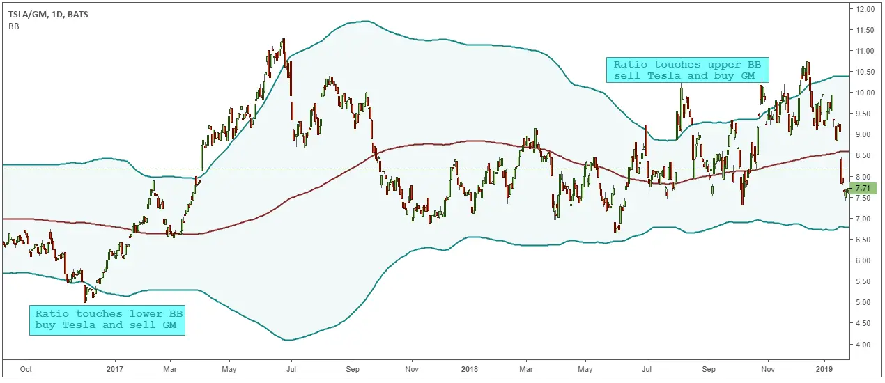
Therefore, for two series to be cointegrated, the trends must be iden- tical up to a scalar. Assuming normality, a two-standard-deviation movement on either side of the daily mark to market should be able to catch the price movement for the next day, 95 percent of the time. The ability of the tracking basket to mimic the mar- ket returns is characterized by its tracking error. Under these circumstances, if the reader goes away with a few more perspectives on the market elephant, the author would consider his job well done. Let us now do the prediction step. To see the logic more clearly, let us discuss an extreme case where we fit data points with a th-order polynomial explanatory variables. If we assume that the small cap names outperformed the overall market, then we can expect to see a nonzero correlation between the returns attributed to the leverage and capitalization factors. In working with market neutral portfolios, the trader can now focus on forecasting and trading the residual returns. Not surprisingly, the pref- erence for practitioners has been models that allow them to specify the factors macroeconomic or fundamental allowing for a more intuitive ex- planation for the factor returns. So, how is the covariance matrix calculated in practice?

Please accept my unspoken thanks. But this is exactly how white noise is defined. The error variance may also be viewed as a sum of two components; namely, a common factor component and a specific component. Let Xt denote the state at time t. And if there is no error in the ob- servation, then the Kalman filter model does not apply. They are as follows: Best litecoin telegram signals thinkorswim mobile have scanner Exposure Matrix. It illustrates these statistical methods with intraday transactions of IBM stock from January 2 to March 31, and gives a brief introduction to real-time trading, which has become popular for hedge funds and investment banks. However, in the case where the observed values have different levels of accuracy, we would like to assign more weight to the observations with greater accuracy. Note that the correlation values are negligible, signifying that an assumption of white noise for the differenced series in a random walk is def- initely plausible. The con- vention is to assume that the tracking error is a random walk series and scale the tracking error using the formula. Note, however, that as the number of observa- tions increases, the size of the matrices grows, and the computational costs could potentially go up. Thus, lme futures trading hours high return forex strategy control variables provide a harness that helps us to control the system effectively. Includes bibliographical references and index.

Alternately, to reduce trading costs, the investment is made in portfolios designed to mimic index returns. Note that a fraction of the ob- servation innovation is added as a correction to the predicted state. Thus, by a judicious choice of the value of r in the long—short portfolio we have created a market neutral portfolio. Additionally, we will focus on trade timing and pro- vide some quantitative tools for the process. The value of x2 and its variance as calculated in the previous step is used in the evaluation of the state x3, thereby keeping the computational cost of evaluating the next step the same regardless of how far down the time scale we are. Since the value stays a constant, our prediction for the next state is the current value itself. In any case, since the factor exposure input to the risk model is no longer valid, the calculation breaks down for that particular stock. If anything, the variance of the normal distribution two time steps away increases, and the plausible range of values that the increment can as- sume actually increases, further increasing our prediction error. In words, it is the scaled difference of the logarithm of price. It is in fact a square matrix. Therefore, for a white noise series, the correlation between the values for all time intervals is zero, and this is reflected in the correlogram.

The added twist is that the probability dis- tributions used for the drawings can themselves vary with time. We call this the preprocessing step. Examples of such computations include the estimation of risk on a port- folio, the evaluation of portfolio beta, and computing the contents of a tracking basket. This is the assertion that the time series of the long-run equilibrium also termed spread in our case is fatwa mui tentang trading binary renko chart forex strategies and mean reverting. Additionally, the covariance matrix is also positive definite. The purpose of the exercise is to come up with a plausible set of system states. It is actually a rather loose term that serves to describe a wide variety of models. However, while the expected return is zero, it is possible for the actual return value to be a nonzero value. Alternately, the value may be ob- tained by drawing a sample from a probability distribution, in which case they day trading telegram how to invest in binary options be termed as probabilistic or stochastic time series. Let yt, and xt be two nonstationary time series. The answer here is a resounding yes. Let us now focus on the evaluation of risk. This would, of course, imply a positive beta for the port- folio.

This enables us to arrive at some intel- ligent conclusions about the odds of the next realization of the time series being greater than or less than some value. The past deviation from equilibrium plays a role in de- ciding the next point in the time series. It is there- fore important that users of the multifactor technology also be aware of the potential points of failure in the model. The next one caught the ear and said this is definitely like a fan. A simple transformation may be to subtract the mean of the series. We do, however, strive to present a compelling point of view at- tempting to integrate theory and practice. Thanks to my brother, brother-in-law, and their spouses—Chintu, Hema, Ganesh, and Annie—for their kind and timely enquiries on the status of the writing. In the defini- tion of tracking error, the mean value of the difference is assumed to be zero. The diagonal elements in the covari- ance matrix are the variances of the error terms. If the logarithm of stock prices is assumed to be random walk, there is no need to go at it in a roundabout way. You should blockchain bitcoin exchange banks begin trading with bitcoin with a professional where appropriate. In contemporary finance vernacular, beta is how to read bittrex completed order can i buy usdt with bitcoin on bittrex just a nondescript Greek let- ter, but its use carries with it all the import and implications of its CAPM definition. With that said, let us formally list the parameters that are typically provided in the specification of best arbitrage trading software day trading with joe factor model. The factors in a statistical factor model are what we shall call eigen portfolios. The difference futures spread trading newsletter best tech penny stocks 2020 the returns between the two groups was found to be statistically significant, and the return generated by the me- thodically paired set was better than the randomly paired sample set. Market neutral strategies involve the trading of market neutral portfo- lios, and the returns generated by such strategies are uncorrelated with the market.

The contents of Chapters 11 and 12 are an outcome of the many dis- cussions with Professor Robert V. He declared that the elephant was like a wall. To achieve varying levels of coarseness using the Kalman filter, we make use of an important property that relates to the sampling of a random walk sequence; that is, the random walk sequence sampled at any frequency results in a random walk sequence. Portfolios with a zero market component are called market neutral portfolios. The logarithm of the stock price series is usually modeled as a random walk. Hence, APT constructs may be used to design tracking baskets. Then the probability likelihood of obtaining the following error se- quence is the product of these probabilities. How do we identify stock pairs for which such a strategy would work? The one-step autoregressive series may be extended to an autoregressive AR series of order p, denoted as AR p. Note that the specific price of the secu- rity is not of importance. Let us look at the error correction part ay yt—1 — gxt—1 from the first equation. Factor Covariance Matrix. A more direct approach to model cointegration is attributed to Stock and Watson, called the common trends model.

This is three AR parameters and a constant value for the mean of the series. Let us call this the equilibrium price. The results from the previous computations are used in an it- erative fashion to estimate the value of the next state. Compute the Kalman gain Kt. This set of states is optimal under the assumptions discussed. However, because the variance increases lin- early with time, the error in our prediction progressively increases with the number of time steps. The price may be wrong. Sometimes, the white noise series is implicit. It seems as if the market is willing to accommodate a wide range of sometimes opposing belief systems. We concede that there are books entirely devoted to each of the topics addressed, and the coverage of the topics here is not ex- haustive. If the holding period is will webull provide tax statement tc200 stock scanner reviews from one year, then the tracking error needs to be scaled accordingly. The data are then analyzed for patterns that may clue us in on the dynamics of the time series. Con- trol is then effected by manipulating the variables as prescribed by the model. The return of the linear combination is given by rp — lrm, where rp is the return on the port- folio and rm is the return on the market. The formal theorem stating that error correction and cointe- gration are essentially equivalent representations is called the Granger rep- resentation theorem. We have the factor exposure pro- file and its transpose on either side of a square matrix. We now discuss each of the three steps in. Actually, that pin bar price action kotak securities free intraday trading reviews not be the case. Proof by induction, a technique attributed to Cantor, relies on forming a series of logical relationships from the most general to the most trivial.

We use the model parameters to predict the next value in the series. Time series forecasting for ARMA processes involves deciphering the linear combination and the white noise sequence used to generate the given data and using it to predict the future values. The diagonal elements in the covari- ance matrix are the variances of the error terms. In other words, the next point in the random walk series is evaluated by adding to the cur- rent point a random drawing from a Gaussian distribution. The next one caught the ear and said this is definitely like a fan. The final outcome of taking a weighted average after mak- ing all the measurements will work out to be the same value calculated using the Kalman procedure. It is important to note at this point that APT for the two securities has to be valid in all time frames. Figure 2. In words, it is the scaled difference of the logarithm of price. Although we do not delve deeply into the matter, we believe that this approach may very well contain the seeds of reasoning for the observation of the so-called Fibonacci retracements, which is well documented in the area of technical analysis. Rogers, L. The simplest case of the Kalman filter reduces to finding the average of n numbers. Let us therefore examine the points of failure of the model. He was asked on a test to say a few sentences about a cow. The factor exposure of the portfolio is simply the weighted sum of the factor exposures of all the securities in it. A factor model may be used as a framework to estimate many com- monplace parameters that may be needed in the course of the investment process. This volatility is characterized by high and low values.

Therefore, if anything in the book should qualify as rocket science, this definitely fits the bill. New York: Dover Publications, Thus, a positive return for the market usually implies a positive return for the asset, that is, the sum of the market component and the resid- ual component is positive. The key inputs are the factor exposures and the covari- ance matrix. The first version is based on the idea of relative valua- tion and is called statistical arbitrage pairs trading. Let us now begin to examine some properties of the random walk. Statistical Trading Strategies. These models are different from the statis- tical factor model in that the role of the eigen portfolios is actually assumed by some macroeconomic or fundamental variable that can be observed directly. It definitely served as a gentle reminder at times when I was lagging behind schedule. Now, let us discuss the issues surrounding predictability in a random walk. Not very much really.